NHL Player Goals by Season AutoRegressive Analysis
Time series data is it's own particular type of beast. It's like that friend who needs a little more attention and to be treated their own special way. One special way to deal with time series data is through the use of a autoregressive modeling (FANCY TERM ALERT!).

An autoregressive model is defined as a regression model that uses a previous period value from a time series dependent variable. It comes in the form of the below equations.
\begin{equation*} y_{t}=\beta_{0}+\beta_{1}y_{t-1}+\epsilon_{t}. \end{equation*}
In this regression model, the response variable in the previous time period has become the predictor. We describe autoregressive by their order. The order of an autoregressive model is the number of preceding values in the series used to predict the value at the present time, e.g. the above equation is written as AR(1). As in a simple linear regression model, autoregressive models are subject to our usual assumptions about errors.
First things first, how do we lag the dependent variable using python? Well, lucky for you I have created a function using python and panda's shift function. The basis from this function comes from Tom Augspurger's Modern Pandas blog (a must read for any heavy pandas user).
def create_lags(input_df, metric, n=5, include_metric_name_in_columns=False):
df = input_df.copy()
frames = [df.groupby('skaterFullName')[metric].shift(i) for i in range(n+1)]
if include_metric_name_in_columns:
keys = [metric] + [metric + '_L%s' % i for i in range(1, n+1)]
else:
keys = ['y'] + ['L%s' % i for i in range(1, n+1)]
df = (pd.concat(frames, axis=1, keys=keys)
.dropna()
)
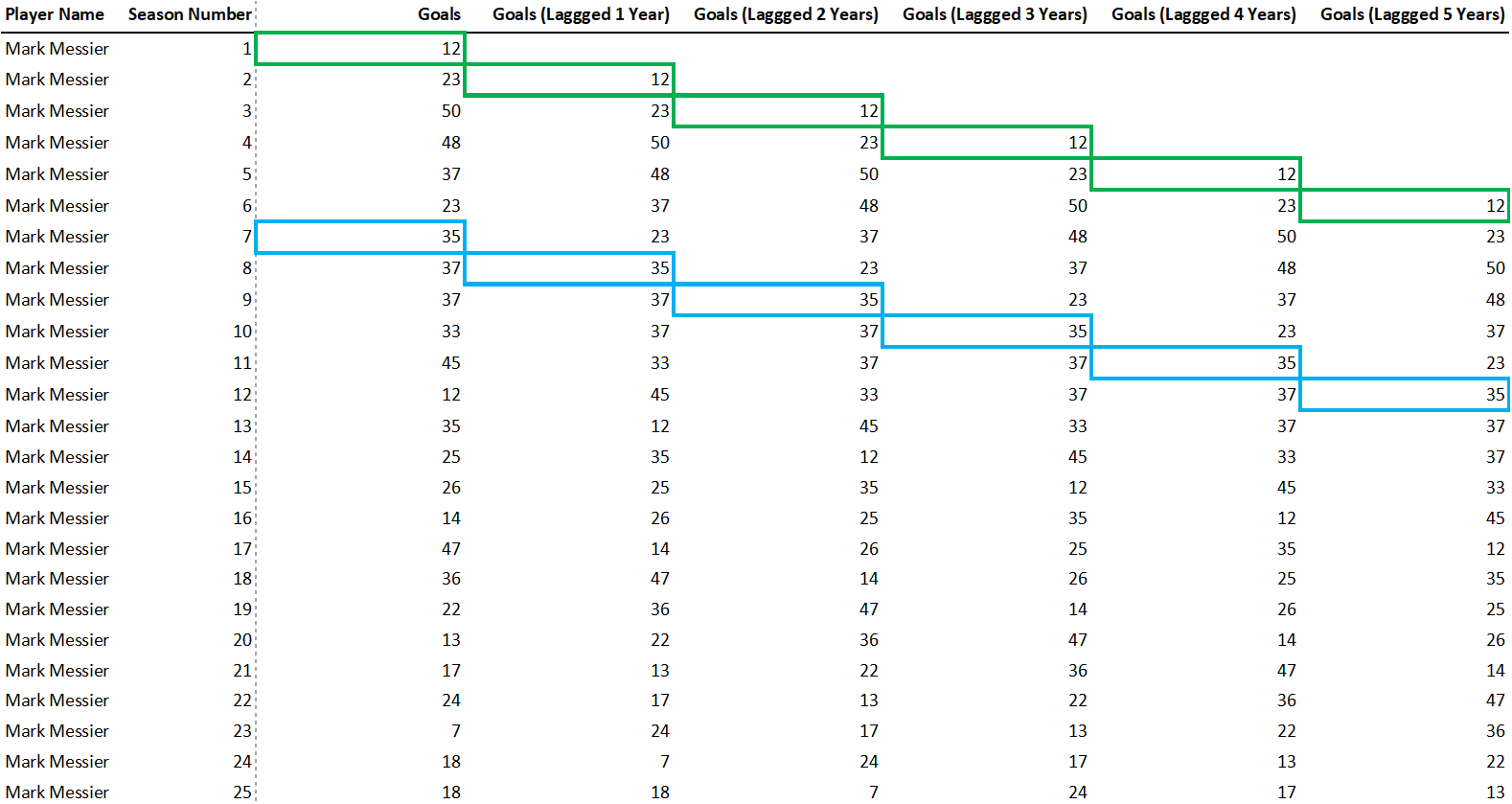
return dfThis function takes in an input_df and metric and lags that variable n times, joining them all together. The resulting dataframe will be a lagged variable. The below table image illustrates how goals would be lagged for Mark Messier. The green boxes show how his rookie year goals are lagged across the next 5 years. The blue boxes show how his 7th year goals are lagged across the next 5 years.
Now let's get to the fun modeling part. First, let's try an AR(3) goals model.
| Dep. Variable: | y | R-squared: | 0.589 |
|---|---|---|---|
| Model: | OLS | Adj. R-squared: | 0.589 |
| Method: | Least Squares | F-statistic: | 6065. |
| Date: | Tue, 02 Jun 2020 | Prob (F-statistic): | 0.00 |
| Time: | 09:19:12 | Log-Likelihood: | -41399. |
| No. Observations: | 12717 | AIC: | 8.281e+04 |
| Df Residuals: | 12713 | BIC: | 8.284e+04 |
| Df Model: | 3 | ||
| Covariance Type: | nonrobust |
| coef | std err | t | P>|t| | [0.025 | 0.975] | |
|---|---|---|---|---|---|---|
| Intercept | 1.2496 | 0.085 | 14.651 | 0.000 | 1.082 | 1.417 |
| L1 | 0.4560 | 0.008 | 53.933 | 0.000 | 0.439 | 0.473 |
| L2 | 0.2154 | 0.009 | 23.877 | 0.000 | 0.198 | 0.233 |
| L3 | 0.1420 | 0.008 | 17.486 | 0.000 | 0.126 | 0.158 |
| Omnibus: | 1599.138 | Durbin-Watson: | 2.097 |
|---|---|---|---|
| Prob(Omnibus): | 0.000 | Jarque-Bera (JB): | 5318.147 |
| Skew: | 0.637 | Prob(JB): | 0.00 |
| Kurtosis: | 5.901 | Cond. No. | 37.3 |
We can see that this model explains roughly 58.9% of the variance of a player's goals. Not a bad result. Interpretation: by knowing a player's last three year's of goals scored we can get make a 58.9% better guess than just guessing the mean goals for all players. All variables have p-value less than 5%, so we can assume they are useful in predicting this years goals. In fact, all variables have a p-value of 0.00%! Let's get a little wild with an AR(5) model.
| Dep. Variable: | y | R-squared: | 0.623 |
|---|---|---|---|
| Model: | OLS | Adj. R-squared: | 0.622 |
| Method: | Least Squares | F-statistic: | 2866. |
| Date: | Tue, 02 Jun 2020 | Prob (F-statistic): | 0.00 |
| Time: | 09:19:12 | Log-Likelihood: | -28028. |
| No. Observations: | 8695 | AIC: | 5.607e+04 |
| Df Residuals: | 8689 | BIC: | 5.611e+04 |
| Df Model: | 5 | ||
| Covariance Type: | nonrobust |
| coef | std err | t | P>|t| | [0.025 | 0.975] | |
|---|---|---|---|---|---|---|
| Intercept | 0.4006 | 0.106 | 3.764 | 0.000 | 0.192 | 0.609 |
| L1 | 0.4161 | 0.010 | 40.694 | 0.000 | 0.396 | 0.436 |
| L2 | 0.2154 | 0.011 | 20.268 | 0.000 | 0.195 | 0.236 |
| L3 | 0.1577 | 0.010 | 15.131 | 0.000 | 0.137 | 0.178 |
| L4 | 0.0625 | 0.010 | 6.088 | 0.000 | 0.042 | 0.083 |
| L5 | 0.0029 | 0.009 | 0.313 | 0.754 | -0.015 | 0.021 |
| Omnibus: | 874.612 | Durbin-Watson: | 2.065 |
|---|---|---|---|
| Prob(Omnibus): | 0.000 | Jarque-Bera (JB): | 2677.525 |
| Skew: | 0.528 | Prob(JB): | 0.00 |
| Kurtosis: | 5.505 | Cond. No. | 53.9 |
This resulted in a 6% increased in our R2, from 0.589 to 0.623. All variables have p-values of 0.00 again. We'll stop a AR(5) because it has good explanatory value and because players typicall re-negoatie contracts after 5 years. This means 5 years will be a good time to use this models to predict next year's goals as a metric for determining their contract value. Let's add a variable for the season number for that player (i.e. their rookie year is 1, their second year is 2, etc.).
| Dep. Variable: | y | R-squared: | 0.632 |
|---|---|---|---|
| Model: | OLS | Adj. R-squared: | 0.632 |
| Method: | Least Squares | F-statistic: | 2486. |
| Date: | Tue, 02 Jun 2020 | Prob (F-statistic): | 0.00 |
| Time: | 09:18:33 | Log-Likelihood: | -27917. |
| No. Observations: | 8695 | AIC: | 5.585e+04 |
| Df Residuals: | 8688 | BIC: | 5.590e+04 |
| Df Model: | 6 | ||
| Covariance Type: | nonrobust |
| coef | std err | t | P>|t| | [0.025 | 0.975] | |
|---|---|---|---|---|---|---|
| Intercept | 3.3540 | 0.224 | 14.987 | 0.000 | 2.915 | 3.793 |
| L1 | 0.4035 | 0.010 | 39.822 | 0.000 | 0.384 | 0.423 |
| L2 | 0.2103 | 0.011 | 20.021 | 0.000 | 0.190 | 0.231 |
| L3 | 0.1575 | 0.010 | 15.314 | 0.000 | 0.137 | 0.178 |
| L4 | 0.0718 | 0.010 | 7.070 | 0.000 | 0.052 | 0.092 |
| L5 | 0.0334 | 0.009 | 3.595 | 0.000 | 0.015 | 0.052 |
| season_number | -0.3491 | 0.023 | -14.948 | 0.000 | -0.395 | -0.303 |
| Omnibus: | 801.168 | Durbin-Watson: | 2.034 |
|---|---|---|---|
| Prob(Omnibus): | 0.000 | Jarque-Bera (JB): | 2548.447 |
| Skew: | 0.470 | Prob(JB): | 0.00 |
| Kurtosis: | 5.480 | Cond. No. | 118. |
Season number is also significant but notice that season number is negative. Does that make sense?
A player's goals usually follows a U-curve as their career progresses, i.e. a player starts with a low number of goals in their first few years, but after gaining some experience they score more as they start hitting their career peak until their goals drop again as age starts to take effect. The below chart illustrates this.
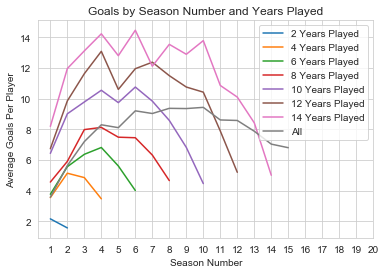
However, our model is only trained on data after a player has 5 years of data. Therefore, the model is picking up on the third leg of that career journey. This explains why we would have a negative coefficient for season_number. If we based the model on all years of players career, we would need to account for that nonlinear relationship, but as we only track players after they have played 5 years, this makes sense. Next let's add games played to our model.
| Dep. Variable: | y | R-squared: | 0.714 |
|---|---|---|---|
| Model: | OLS | Adj. R-squared: | 0.714 |
| Method: | Least Squares | F-statistic: | 3105. |
| Date: | Tue, 02 Jun 2020 | Prob (F-statistic): | 0.00 |
| Time: | 09:18:33 | Log-Likelihood: | -26814. |
| No. Observations: | 8695 | AIC: | 5.364e+04 |
| Df Residuals: | 8687 | BIC: | 5.370e+04 |
| Df Model: | 7 | ||
| Covariance Type: | nonrobust |
| coef | std err | t | P>|t| | [0.025 | 0.975] | |
|---|---|---|---|---|---|---|
| Intercept | -3.6290 | 0.241 | -15.030 | 0.000 | -4.102 | -3.156 |
| L1 | 0.3281 | 0.009 | 36.251 | 0.000 | 0.310 | 0.346 |
| L2 | 0.1919 | 0.009 | 20.722 | 0.000 | 0.174 | 0.210 |
| L3 | 0.1460 | 0.009 | 16.100 | 0.000 | 0.128 | 0.164 |
| L4 | 0.0729 | 0.009 | 8.143 | 0.000 | 0.055 | 0.090 |
| L5 | 0.0417 | 0.008 | 5.092 | 0.000 | 0.026 | 0.058 |
| season_number | -0.3619 | 0.021 | -17.588 | 0.000 | -0.402 | -0.322 |
| gamesPlayed | 0.1348 | 0.003 | 50.087 | 0.000 | 0.130 | 0.140 |
| Omnibus: | 1208.057 | Durbin-Watson: | 1.879 |
|---|---|---|---|
| Prob(Omnibus): | 0.000 | Jarque-Bera (JB): | 3082.868 |
| Skew: | 0.782 | Prob(JB): | 0.00 |
| Kurtosis: | 5.463 | Cond. No. | 302. |
Another significant variable. The F-statistic is still very large as well, illustrating our model as a whole is solid. Let's keep moving forward (pun intended) and add a variable for position.
| Dep. Variable: | y | R-squared: | 0.718 |
|---|---|---|---|
| Model: | OLS | Adj. R-squared: | 0.717 |
| Method: | Least Squares | F-statistic: | 2207. |
| Date: | Tue, 02 Jun 2020 | Prob (F-statistic): | 0.00 |
| Time: | 09:18:33 | Log-Likelihood: | -26766. |
| No. Observations: | 8695 | AIC: | 5.355e+04 |
| Df Residuals: | 8684 | BIC: | 5.363e+04 |
| Df Model: | 10 | ||
| Covariance Type: | nonrobust |
| coef | std err | t | P>|t| | [0.025 | 0.975] | |
|---|---|---|---|---|---|---|
| Intercept | -2.9364 | 0.267 | -11.009 | 0.000 | -3.459 | -2.414 |
| C(positionCode)[T.D] | -1.4347 | 0.165 | -8.695 | 0.000 | -1.758 | -1.111 |
| C(positionCode)[T.L] | -0.2017 | 0.169 | -1.197 | 0.231 | -0.532 | 0.129 |
| C(positionCode)[T.R] | 0.0742 | 0.169 | 0.439 | 0.661 | -0.257 | 0.406 |
| L1 | 0.3162 | 0.009 | 34.813 | 0.000 | 0.298 | 0.334 |
| L2 | 0.1810 | 0.009 | 19.510 | 0.000 | 0.163 | 0.199 |
| L3 | 0.1369 | 0.009 | 15.095 | 0.000 | 0.119 | 0.155 |
| L4 | 0.0660 | 0.009 | 7.391 | 0.000 | 0.049 | 0.084 |
| L5 | 0.0371 | 0.008 | 4.548 | 0.000 | 0.021 | 0.053 |
| season_number | -0.3473 | 0.021 | -16.909 | 0.000 | -0.388 | -0.307 |
| gamesPlayed | 0.1381 | 0.003 | 51.119 | 0.000 | 0.133 | 0.143 |
| Omnibus: | 1204.406 | Durbin-Watson: | 1.873 |
|---|---|---|---|
| Prob(Omnibus): | 0.000 | Jarque-Bera (JB): | 3054.431 |
| Skew: | 0.782 | Prob(JB): | 0.00 |
| Kurtosis: | 5.447 | Cond. No. | 375. |
Only being a defenseman is significant in this model. Let's transform that column to only differentiate between Forward's and Defenseman.
| Dep. Variable: | y | R-squared: | 0.718 |
|---|---|---|---|
| Model: | OLS | Adj. R-squared: | 0.717 |
| Method: | Least Squares | F-statistic: | 2758. |
| Date: | Tue, 02 Jun 2020 | Prob (F-statistic): | 0.00 |
| Time: | 09:18:33 | Log-Likelihood: | -26767. |
| No. Observations: | 8695 | AIC: | 5.355e+04 |
| Df Residuals: | 8686 | BIC: | 5.362e+04 |
| Df Model: | 8 | ||
| Covariance Type: | nonrobust |
| coef | std err | t | P>|t| | [0.025 | 0.975] | |
|---|---|---|---|---|---|---|
| Intercept | -4.3846 | 0.252 | -17.376 | 0.000 | -4.879 | -3.890 |
| C(positionCode)[T.F] | 1.3897 | 0.142 | 9.756 | 0.000 | 1.110 | 1.669 |
| L1 | 0.3164 | 0.009 | 34.840 | 0.000 | 0.299 | 0.334 |
| L2 | 0.1810 | 0.009 | 19.518 | 0.000 | 0.163 | 0.199 |
| L3 | 0.1368 | 0.009 | 15.095 | 0.000 | 0.119 | 0.155 |
| L4 | 0.0662 | 0.009 | 7.408 | 0.000 | 0.049 | 0.084 |
| L5 | 0.0373 | 0.008 | 4.570 | 0.000 | 0.021 | 0.053 |
| season_number | -0.3464 | 0.021 | -16.879 | 0.000 | -0.387 | -0.306 |
| gamesPlayed | 0.1381 | 0.003 | 51.187 | 0.000 | 0.133 | 0.143 |
| Omnibus: | 1208.329 | Durbin-Watson: | 1.873 |
|---|---|---|---|
| Prob(Omnibus): | 0.000 | Jarque-Bera (JB): | 3073.302 |
| Skew: | 0.783 | Prob(JB): | 0.00 |
| Kurtosis: | 5.456 | Cond. No. | 324. |
Our final model is looking great. We've increased our R2 22% from our first model (0.589 to 0.718). Our F-statistic is large and all of our features are significant. Let's interpret them one-by-one by analyzing each by sign, size and significance. All variables are significant so we'll focus on the first two.
Intercept
Our model assumes you have scored -4.3846 if all other variables are 0. This doesn't make a ton of sense as you can score negative goals, but it is interpretable in the context of other variables. Basically, our model is saying you don't automatically start scoring goals, but you have to traverse -4.4 theoretical goals before we give you any real ones. We'll look at gamesPlayed next further.
gamesPlayed
Our gamesPlayed coefficient is 0.1381. The sign is positive meaning our model thinks you'll score more goals as you play more games (duh!). More specifically, each goal you play will allot 0.1381 goals. Fractional goals are nonsense, but in a more literal context, every 7 games we'll score a goal according to our model (ceterus paribus).
C(positionCode)[T.F]
Our model allots 1.3897 goals per season if you are forward. Basically it will give you more goals for being a forward than being a defenseman. This seems low to me as forwards average about 14 goals per year (assuming 82 games played) in our dataset, while defenseman only average 5. But, close enough, can't win 'em all.
L1
Now let's dig into the autoregressive variables. Goals from last year's (L1) has a coefficient of 0.3164. This means we will add ~32% of last year's goal to our total.
L2
We will add 18% of the player's goals from two years ago to our total. The cool thing about this model is the size of each lagged variable's coefficient is smaller as we get further from the current year. This is intuitive as players performance from last year is more likely to be impactful on this year's performance than their performance from 5 years ago.
L3
We will add 13.7% of the player's goals from three years ago to our total.
L4
We will add 6.6% of the player's goals from four years ago to our total.
L5
We will add 3.7% of the player's goals from five years ago to our total.
Wrapping Up
Overall this was a really fun model to analyze. There are definitely some issues with the errors I will analyze in further posts, but good times good times nonetheless.
Thanks for reading!