NCAA Tournament Seed Matchup Bayesian Modeling
We're coming up to that time of year where the NCAA tournament is almost upon us!
Filling out your brackets can be an overwhelming process, even when you have watched a lot of college hoops over the year. For the first round especially, it's tough to evaluate 64 teams separately. Luckily, we have our good friend statistics to help us out! In this blog, we'll use a historical game results from 1985 (the first year the tournament had 64 teams) to 2019 (our last year of data) to create distributions for a binomial model probability of winning for the higher ranked team.
Our strategy will be to use Bayesian modeling to determine a higher seed's probability of winning. This will allow even the most passive fan to get some good W's in their bracket. We'll use the beta-binomial distribution using a Bayesian conjugate update to dervive our final beta distributions of binomial win probabilities. We're going to gloss over the mechanics behind the distribution for the sake of time (and to avoid losing all readers!) but it's a greater introduction to Bayesian statistics if you're interested.
The reason we're using distributions and not soley assuming the historical win rates is that historical win rates aren't necessarily a proper indicator for future win rates. By using the beta-binomial conjugate family we can create a confidence interval for this metric. Over time the win rate will change but should always be within this interval if we do our job right.
First, we'll need some good ole data to work with. Since this is a smaller project, rather than using my personal favorite scraping tool, Scrapy, I used urllib and lxml. You can find my spider here where I scraped sports-reference.com.
This gave us a dataset looking like this.
| year | region | round | home_seed | home_team | home_score | away_seed | away_team | away_score | seed_matchup | winner | seed_result | |
|---|---|---|---|---|---|---|---|---|---|---|---|---|
| 0 | 1985 | east | 1 | 1 | Georgetown | 68 | 16 | Lehigh | 43 | 01v16 | home_team | higher_seed_win |
| 1 | 1985 | east | 1 | 8 | Temple | 60 | 9 | Virginia Tech | 57 | 08v09 | home_team | higher_seed_win |
| 2 | 1985 | east | 1 | 5 | SMU | 85 | 12 | Old Dominion | 68 | 05v12 | home_team | higher_seed_win |
| 3 | 1985 | east | 1 | 4 | Loyola (IL) | 59 | 13 | Iona | 58 | 04v13 | home_team | higher_seed_win |
| 4 | 1985 | east | 1 | 6 | Georgia | 67 | 11 | Wichita State | 59 | 06v11 | home_team | higher_seed_win |
Next, we'll do some data checks to make sure everything is good and then some data cleaning too. These checks ensure we have the proper number of games and there are no ties.
def data_checks(df):
    # check games total
    if not(63 * (END_YEAR - START_YEAR + 1) == df.shape[0]):
        return {"result": "failed", "test": "games total"}

    # no ties
    if not(df.loc[df.home_score == df.away_score, ].empty):
        return {"result": "failed", "test": "no ties"}

    return {"result": "passed"}
Then we'll take this data and filter for only the first round matchups using the below code.
mask = df.loc[:, 'round'] == 1
first_round_matchups = (df.loc[mask, 'seed_matchup']
    .drop_duplicates()
    .sort_values()
    .tolist()
)


models = dict()

for matchup in first_round_matchups:
    df_matchup = df.loc[df.seed_matchup == matchup, ]

    higher_seed, lower_seed = list(map(int, matchup.split('v')))

    model = BayesBetaBinomial(matchup, a_prior=lower_seed, b_prior=higher_seed)

    x = sum(df_matchup.seed_result == 'higher_seed_win')
    n = df_matchup.shape[0]
    model.update(x, n)

    title = f'{higher_seed} vs {lower_seed} Seed Matchups - Bayesian Posterior Distribution'
    ax = model.plot_posterior(title)
    plt.savefig(f'data/{matchup}_posterior_distribution.png')
    plt.show()

    models[matchup] = model
The models used are instances of the BayesBetaBinomial class I wrote to calculate prior and posterior distributions, which you can find here.
Now that we have our models, let's can clean this up and summarize it into the data frame shown below to dive into the results a bit.
| Seed Matchup | Higher Seed Wins | Lower Seed Wins | Higher Seed Win Pct | Higher Seed Win Pct Posterior Mean | Higher Seed Win Pct Lower Bound | Higher Seed Win Pct Upper Bound | Confidence Interval Band |
|---|---|---|---|---|---|---|---|
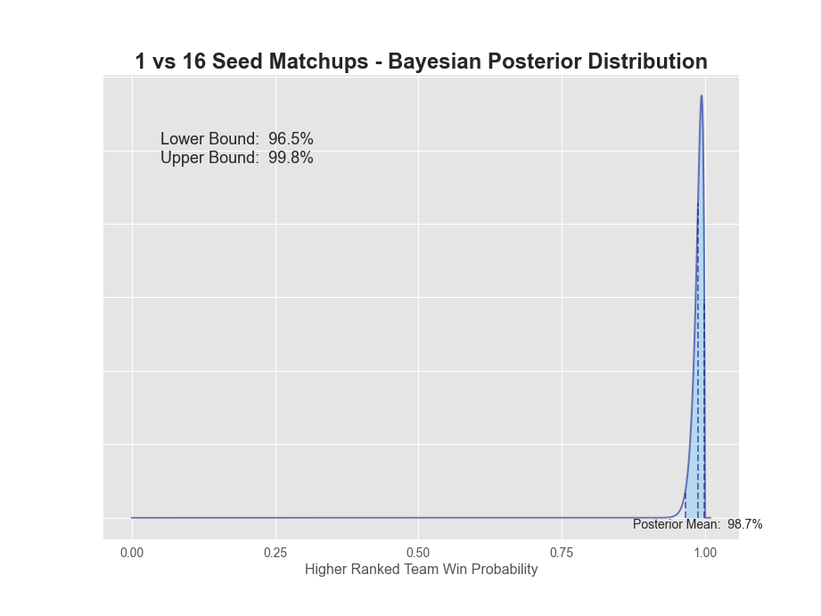
| 01v16 | 139 | 1 | 99.3% | 98.7% | 96.5% | 99.8% | 3.4% |
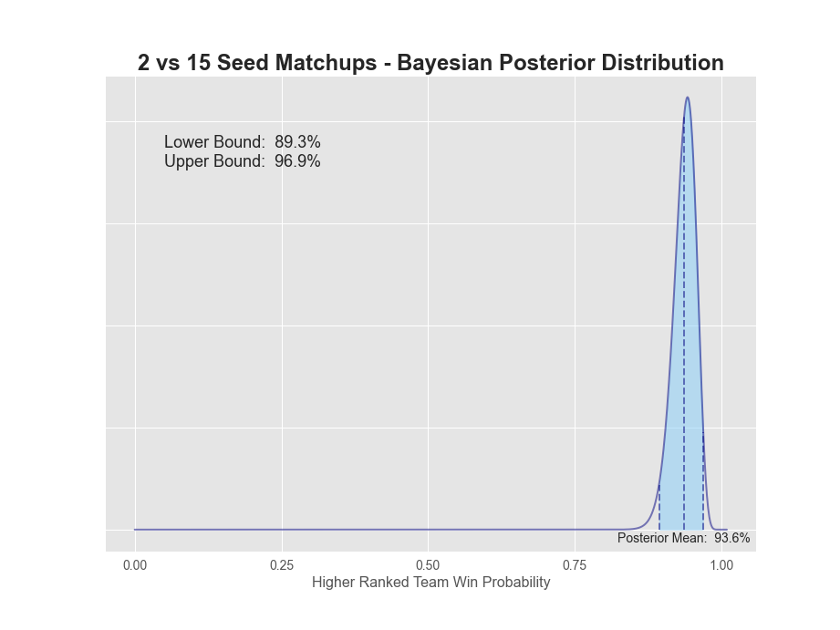
| 02v15 | 132 | 8 | 94.3% | 93.6% | 89.3% | 96.9% | 7.6% |
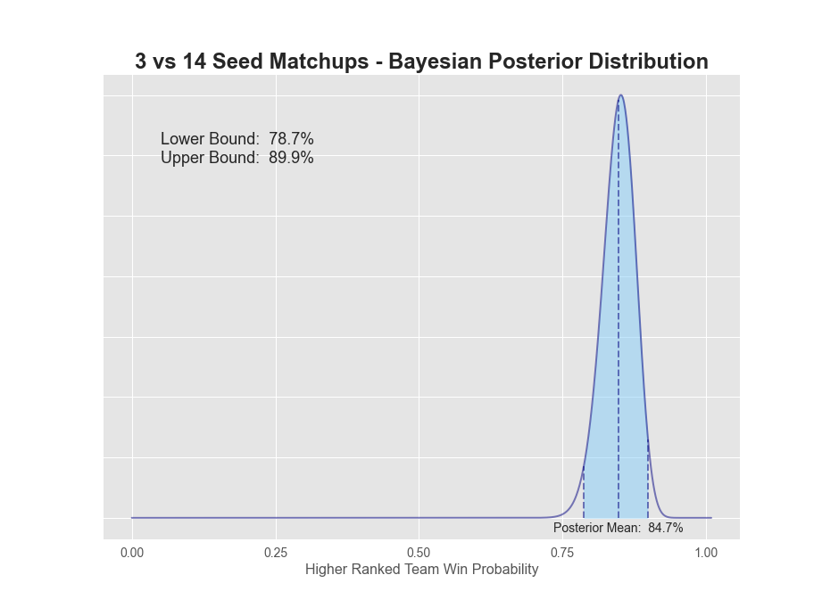
| 03v14 | 119 | 21 | 85.0% | 84.7% | 78.7% | 89.9% | 11.2% |
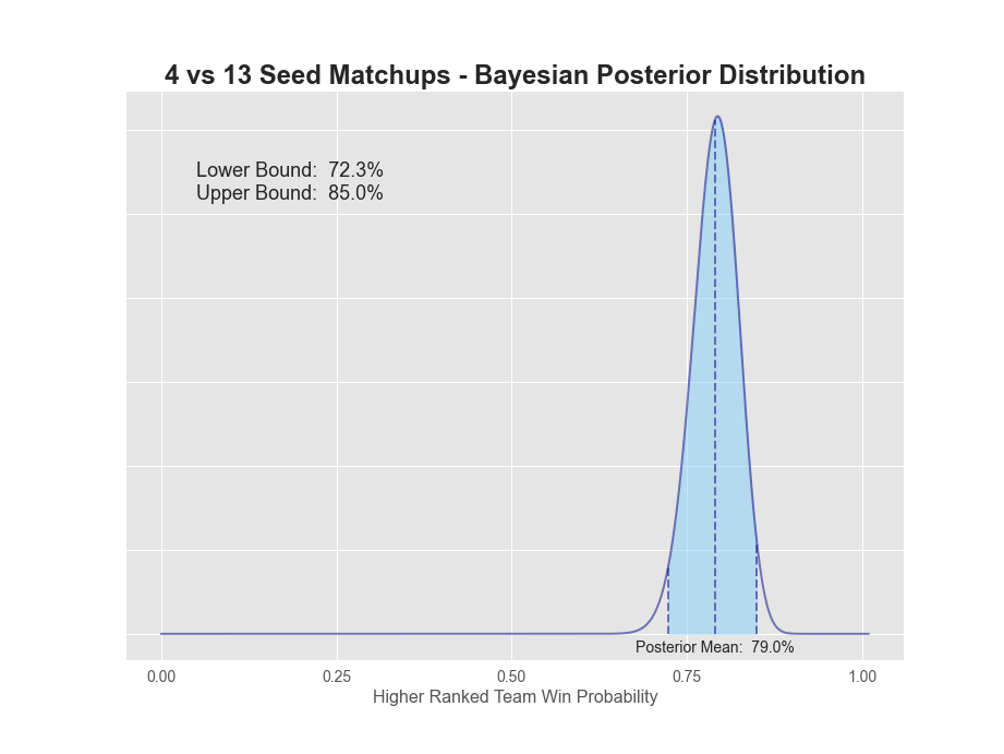
| 04v13 | 111 | 29 | 79.3% | 79.0% | 72.3% | 85.0% | 12.7% |
| 05v12 | 90 | 50 | 64.3% | 65.0% | 57.4% | 72.2% | 14.9% |
| 06v11 | 88 | 52 | 62.9% | 63.1% | 55.4% | 70.4% | 15.0% |
| 07v10 | 85 | 55 | 60.7% | 60.5% | 52.8% | 68.0% | 15.2% |
| 08v09 | 68 | 72 | 48.6% | 49.0% | 41.3% | 56.8% | 15.6% |
Clearly, the higher the seed, the higher the expected win percentage as shown by the Higher Seed Win Pct Posterior Mean metric.
We can also see that our confidence interval gets larger as the seeds become closer, meaning we have less certainty of the true win probability for 8v9 matchups compared to 1v16 matchups.
This pretty little visual shows the results between matchups even more clearly.
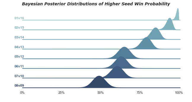
1v16 matchups have a 98.7% probability that the 1-seed will win. The extreme value here is not surprising given there's only been 1 time in history the 16-seed has won (UMBC over Baltimore in 2018). 2-seeds have a 93.6% chance of winning, while 3-seeds dropped down to only 84.7%. 5 through 7 seeds all seem to be in the mid to low 60s, while 8v9 is a coin flip. A more detailed plot of each posterior can be found below.
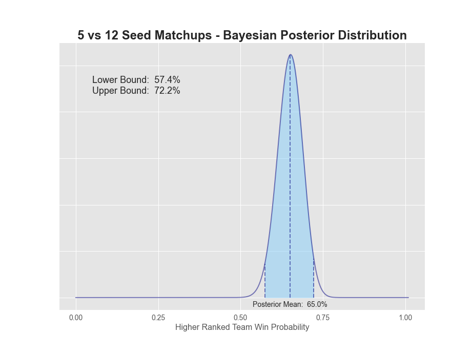

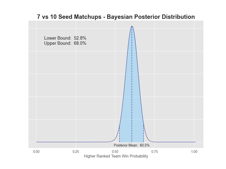
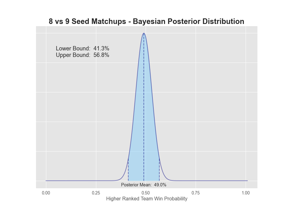
So what are our takeaways? Clearly, it's best to have all 1-seeds, 2-seeds and arguably 3-seeds winning all four games respectively in the first round. 4-seeds are closer to 75%, so you'd want to dig into those matchups for an upset or two. Finally, 5-8 seeds all have lower than a 65% chance or less of winning, so that's where we really want to focus our research.
Good luck with your brackets! Hopefully this helps in your selections. The full analysis can be found in my sport analysis repo here. If you want any other seed matchup distributions, feel free to contact me!
Thanks for reading!