Damian Lillard's NBA Bubble Performance T-Test
Damian Lillard destroyed it in the bubble.
As the unanimously voted seeding games Bubble MVP, Lillard averaged 33 points, 8 assists, and 4 rebounds over the seeding games and the playoffs. He also lead the Blazers to a playoff spots with a win in the playoff game over Memphis, overcoming a three and a half game deficit entering the bubble.
While some of players claimed the bubble was a difficult experience (except for Steven Adams 😂😂😂) Lillard claimed that the bubble was "way easier" to him personally since there were less distractions. See the clip below.
Dame says NBA games were "way easier" in the bubble.
— ESPN (@espn) December 2, 2020
(via @Dame_Lillard, @fatjoe) pic.twitter.com/3aDxPvLKtl
Having personally completed a specialization in Statistics from Duke, I wanted to exercise my hypothesis testing skills, and this seemed like the perfect opportunity to do so.
Duke's stat's department has written an awesome R package called statsr. This package has functions for almost every statistical test. I decided I'd recreate the single mean, hypothesis test under both the theoretical and simulation methods in a python class.
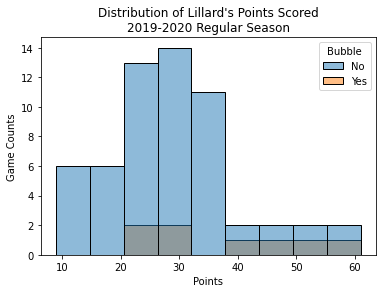
We'll compare only his seeding game performance in the bubble and not the playoff games, the reasoning being that the playoffs are a different beast altogether and they faced the Lakers aka the future champs. Let's look at the distribution of games in the regular season pre-bubble and in-bubble.
| Playoffs | Bubble | PTS | AST | STL | TRB |
|---|---|---|---|---|---|
| Regular Season | Pre | 28.9 | 7.8 | 1.0 | 4.3 |
| In | 37.6 | 9.6 | 1.4 | 4.2 | |
| Playoffs | In | 24.2 | 4.2 | 0.5 | 3.5 |
We can see that his regular season game scoring distribution ranges from 10-60 and has a mean of 28.9, while his regular season bubble average points total was 37.6. His points have a standard deviation of 11.8 points with a right skew - unsurprising given points cannot be negative. Our an effect size for pre-bubble vs buble is 8.7, rather large considering the median point differential for an NBA games is usually around 8 or 9.
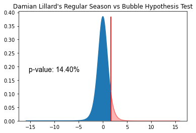
Let's run our first single mean, one-sided hypothesis using the theoretical method. I linked the class here, as it's very lengthy if you're curious. The below visual shows the results of the test and the relevant summary statistics.
| mu | n | std | |
|---|---|---|---|
| Sample 1 (Pre-Bubble) | 28.91 | 58 | 11.09 |
| Sample 2 (In-Bubble) | 37.62 | 8 | 14.40 |
As we talked about above, our effect size was 8.7 pts, while our standard error was 5.3. This gives us a t-statistic of 1.64 with a corresponding p-value of 0.144. While this is a small p-value, it is well above the industry standard alpha of 0.05.
Now, one might be tempted to write off Lillard's claim and say it was a statistically insignificant streak. But, we being no ordinary statisticians, want to look deeper at what's going on. After all, an effect size of 8.7 points is not insignificant in an NBA game. We can see that clearly we don't have many samples for the seeding bubble games (only 8 games). Since we have a small sample size and skewed distribution, we should be using the simulation method of hypothesis testing.
We can do so using the simulation class method in our hypothesis testing python class.
By doing so, we find obtain a p-value of 0.032.
The below shows the distribution of the simulated sample differences between the two simulation means.
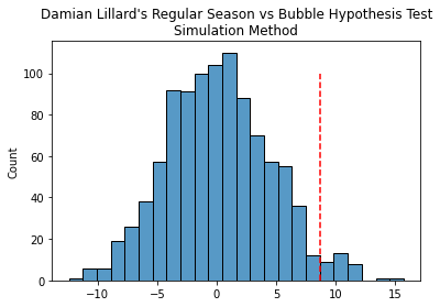
The below visual is centered around zero, as we would expect no difference between playing in the bubble or not. The actual sample test stat is at the red line, and we can see very few simulated samples above it. Thus, under appropriate an sample sizing using the simulation method, we find that Lillard's performance was statistically significant. We can therefore agree with Lillard, that for him, the bubble was a very productive environemnt.